Speed Distribution

A sample of a gas is made of a large number of particles. For example, 4.002 grams (the atomic mass) of Helium used in a blimp has 6.02 × 10²³ (Avogadro's Number) individual atoms of helium which is known as a mole. These particles are not all moving with the same speed – they have a distribution of speeds. Any one particle could be moving very fast or very slow. This distribution of speeds is greatly affected by the temperature of the gas. Hot gases are moving “faster” and cold gases are moving “slower”. The entire distribution of speeds is shifted by changes in temperature.

While it is not necessary for the lab to know the mathematical equation, it is important to note a few general features of the Maxwell distribution:

• The distribution has a crude “bell-shape” which peaks at v_mp = (2kT/m)^1/2, the most probable velocity.
• The exact shape of the distribution is not symmetric. There is a high-speed tail to the distribution.
• The average velocity (speed and direction) is zero. The magnitude of the average velocity v_avg is not found at the peak, but a little past it because of the high-speed tail.

The simulation of the distribution below allows you to animate certain velocity ranges of the particles.

Note that the distribution is a function of the particle mass, thus it is different for each type of gas. The Hydrogen curve will be broader and wider than the distribution of a more massive gas like Carbon Dioxide. The mass of a gas particle can be conveniently expressed in terms of atomic mass units u = 1.66 × 10^-27 kg. A particle has roughly 1 u for each proton or neutron in an atom. Thus, a methane (CH₄) molecule would have a mass of 16 u (12 for carbon which has 6 protons and 6 neutrons and 4 for hydrogen which only has a proton). One mole of methane would have a mass of approximately 16 g (16.0429 actually) and contain 6.02 x 10²³ molecules.

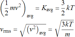
Statistical Mechanics is the branch of physics concerned with relating the microscopic behavior of the particles of the gas to the macroscopic quantities that we measure. It uses a value of velocity slightly larger than v_avg to characterize the distribution known as the root mean square v_rms. For the purpose of this lab, these two values will be used interchangeably. This distribution parameter is directly related to temperature T and mass m of the gas particles. The result from statistical mechanics states that the average kinetic (motion) energy of a particle is proportional to the temperature which allows one to solve for the velocity which is the root of the average square.

RMS Speed of a Gas Molecule

Imagine a volume of gas at the top of a planet’s atmosphere. The gas will have a range of velocities described by the Maxwell distribution. If a particle is moving sufficiently fast (i.e. with a speed greater than the escape velocity) and moving away from the planet, it can escape into space. If the escape velocity is low enough, the gas will be depleted fairly quickly. However, typically the escape speed is very far into the high-speed tail of the Maxwell distribution so only a very few particles will be able to escape. But once these particles are lost, the high-speed tail will be replenished and then lost again. Thus, even if the escape speed is well into the high-speed tail, it can slowly “bleed off” the atmosphere. The constitution of planetary atmospheres has been determined by the interplay between escape velocity and the Maxwell distribution over the 4.6 billion year history of our solar system.